Support Vector Machine – SVM From Scratch Python

In the 1960s, Support vector Machine (SVM) known as supervised machine learning classification was first developed, and later refined in the 1990s which has become extremely popular nowadays owing to its extremely efficient results. The SVM is a supervised algorithm is capable of performing classification, regression, and outlier detection. But, it is widely used in classification objectives. SVM is known as a fast and dependable classification algorithm that performs well even on less amount of data. Let’s begin today’s tutorial on SVM from scratch python.

HOW SVM WORKS ?

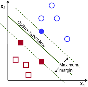
SVM finds the best N-dimensional hyperplane in space that classifies the data points into distinct classes. Support Vector Machines uses the concept of ‘Support Vectors‘, which are the closest points to the hyperplane. A hyperplane is constructed in such a way that distance to the nearest element(support vectors) is the largest. The better the gap, the better the classifier works.

The line (in 2 input feature) or plane (in 3 input feature) is known as a decision boundary. Every new data from test data will be classified according to this decision boundary. The equation of the hyperplane in the ‘M’ dimension :

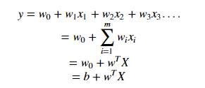
where,

Wi = vectors(W0,W1,W2,W3……Wm)

b = biased term (W0)

X = variables.

The point above or on the hyperplane will be classified as class +1, and the point below the hyperplane will be classified as class -1.

SVM IN NON-LINEAR DATA

SVM can also conduct non-linear classification.

For the above dataset, it is obvious that it is not possible to draw a linear margin to divide the data sets. In such cases, we use the kernel concept.

SVM works on mapping data to higher dimensional feature space so that data points can be categorized even when the data aren’t otherwise linearly separable. SVM finds mapping function to convert 2D input space into 3D output space. In the above condition, we start by adding Y-axis with an idea of moving dataset into higher dimension.. So, we can draw a graph where the y-axis will be the square of data points of the X-axis.

And now, the data are two dimensional, we can draw a Support Vector Classifier that classifies the dataset into two distinct regions. Now, let’s draw a support vector classifier.

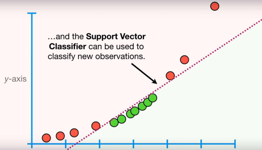
This example is taken from Statquest.

HOW TO TRANSFORM DATA ??

SVM uses a kernel function to draw Support Vector Classifier in a higher dimension. Types of Kernel Functions are :

1.Linear
2.Polynomial
3.Radial Basis Function(rbf)

In the above example, we have used a polynomial kernel function which has a parameter d (degree of polynomial). Kernel systematically increases the degree of the polynomial and the relationship between each pair of observation are used to find Support Vector Classifier. We also use cross-validation to find the good value of d.

Radial Basis Function Kernel

Widely used kernel in SVM, we will be discussing radial basis Function Kernel in this tutorial for SVM from Scratch Python. Radial kernel finds a Support vector Classifier in infinite dimensions. Radial kernel behaves like the Weighted Nearest Neighbour model that means closest observation will have more influence on classifying new data.

SOFT MARGIN – SVM

In this method, SVM makes some incorrect classification and tries to balance the tradeoff between finding the line that maximizes the margin and minimizes misclassification. The level of misclassification tolerance is defined as a hyperparameter termed as a penalty- ‘C’.

For large values of C, the optimization will choose a smaller-margin hyperplane if that hyperplane does a better job of getting all the training points classified correctly. Conversely, a very small value of C will cause the optimizer to look for a larger-margin separating hyperplane, even if that hyperplane misclassifies more points. For very tiny values of C, you should get misclassified examples, often even if your training data is linearly separable.

Due to the presence of some outliers, the hyperplane can’t classify the data points region correctly. In this case, we use a soft margin & C hyperparameter.

SVM IMPLEMENTATION IN PYTHON

In this tutorial, we will be using to implement our SVM algorithm is the Iris dataset. You can download it from this link. Since the Iris dataset has three classes. Also, there are four features available for us to use. We will be using only two features, i.e Sepal length, and Sepal Width.

BONUS – SVM FROM SCRATCH PYTHON!!

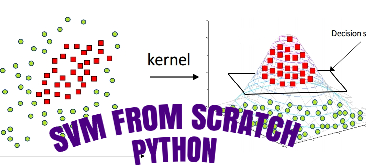
Kernel Trick: Earlier, we had studied SVM classifying non-linear datasets by increasing the dimension of data. When we map data to a higher dimension, there are chances that we may overfit the model. Kernel trick actually refers to using efficient and less expensive ways to transform data into higher dimensions.

Kernel function only calculates relationship between every pair of points as if they are in the higher dimensions; they don’t actually do the transformation. This trick , calculating the high dimensional relationships without actually transforming data to the higher dimension, is called the Kernel Trick.